2-D Beam

2-D Elasticity Solution in a Beam

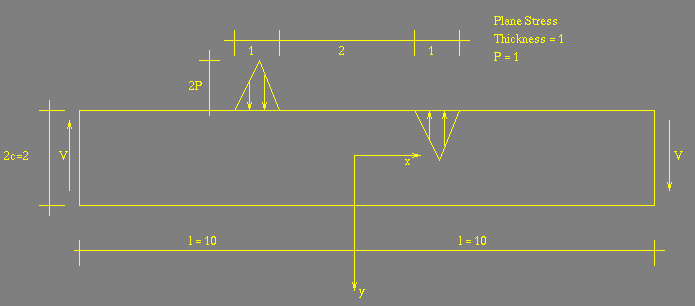
A beam of length 20 and depth 2 is loaded by two triangularly distributed loads along the upper chord. The aspect ratio of the beam is 10 and is thus normally considered to be just barely within the purview of Bernoulli-Euler beam theory. The two loads distributions are statically equivalent to two point forces of magnitude P acting at x=-1.5 and x=1.5 for y = -1 -- one acting up and the other down.

If one assumes the beam is supported by appropriately distribued shear forces on the ends with no normal loads then the analytic solution to this problem can be constructed using a Fourier series in x and a hyperbolic cosine/sine function in y as outlined in Timoshenko and Goodier "Theory of Elasticity" Art. 24.

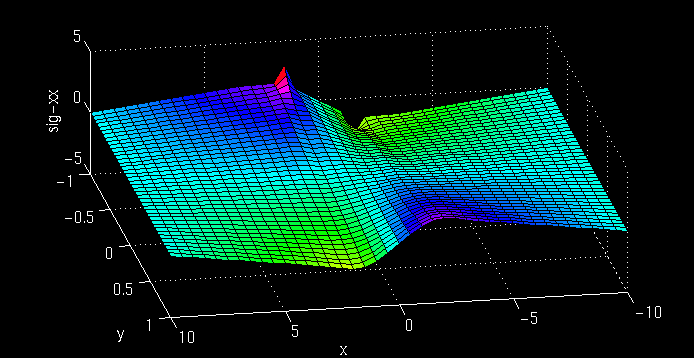
Shown below are the stress fields for the bending stress sigma-xx, the through thickness stress sigma-yy, and the shear stress sigma-xy. N.B. the figures shown below are flipped with respect to the figure above; so pay attention to coordinate values of the points.

Notice how the lower chord displays the usual My/I type of bending stresses, but that this behavior breaks down significantly as one approaches the upper chord.

Notice that the through thickness stresses are non-trivial in the critical regions of the beam and should not be ignored in failure analysis.

Here again, notice how through much of the beam there is a parabolic shear stress distribution as the elementary Bernoulli-Euler theory indicates. However, in the critical region of the beam, the shears are non-trivial and depart significantly from the elementary theory.

Driver file

     N = 50;                %Number of Fourier modes
     c = 1;                 % Half depth
     l = 10;                % Half length
     x = -l:l/20:l;         % x discetization
     y = -c:c/20:c;         % y discetization
     [X,Y]=meshgrid(x,y);
     P = 1;                 % Unit Load
     sigxx = zeros(41,41);  % Initialize stresses
     sigxy = zeros(41,41);  % Initialize stresses
     sigyy = zeros(41,41);  % Initialize stresses
     for m = 1:N            % Loop over Fourier modes
     
       a = m*pi/l;
       A = (8*P/(l*a*a))*(sin(a) + sin(2*a) - 2*sin(1.5*a));   % Fourier Amp
     
        [sx,sy,sxy] = sig(X,Y,a,c,A);   % Compute contribution to stress
     
        sigxx = sigxx + sx;             % Add up
        sigyy = sigyy + sy;             % Add up
        sigxy = sigxy + sxy;            % Add up


     end
     
     surf(X,Y,sigxx)                    % Plot sig-xx (Change for other components)

Stress Evaluation file

       function [sxx,syy,sxy] = sig(x,y,a,c,A)
       %
       % Given a points x and y, a Fourier amplitude A, a half depth c,
       % and a Fourier frequency a, this routine computes the stresses
       % associated with this Fourier mode.
       %
       % Usage  [sxx,syy,sxy] = sig(x,y,a,c,A)
       %
       ac = a*c;
       c = cosh(ac);
       s = sinh(ac);
       sy = sinh(a*y);
       cy = cosh(a*y);
       d1 = 1.0/(sinh(2*ac)+2*ac);
       d2 = 1.0/(sinh(2*ac)-2*ac);
       sxx =  A*( (ac*c - s)*cy - a*y.*sy*s ).*sin(a*x)*d1 ...
            - A*( (ac*s - c)*sy - a*y.*cy*c ).*sin(a*x)*d2;
       syy = -A*( (ac*c + s)*cy - a*y.*sy*s ).*sin(a*x)*d1 ...
            + A*( (ac*s + c)*sy - a*y.*cy*c ).*sin(a*x)*d2;
       sxy = -A*( ac*c*sy - a*y.*cy*s ).*cos(a*x)*d1 ...
            + A*( ac*s*cy - a*y.*sy*c ).*cos(a*x)*d2;